| |||||||||||||||||
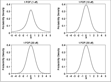
| Probability Density Function | The formula for the probability density function of the t distribution is![f(x) = (1 + x**2/nu)**(-(nu+1)/2)/[B(0.5,0.5*nu)*SQRT(nu)]](http://www.itl.nist.gov/div898/handbook/eda/section3/eqns/tpdf.gif) where  is the beta function and is the beta function and  is a positive integer shape parameter. The formula for the beta function is is a positive integer shape parameter. The formula for the beta function is In a testing context, the t distribution is treated as a "standardized distribution" (i.e., no location or scale parameters). However, in a distributional modeling context (as with other probability distributions), the t distribution itself can be transformed with alocation parameter,  , and a scale parameter, , and a scale parameter,  . .The following is the plot of the t probability density function for 4 different values of the shape parameter.  These plots all have a similar shape. The difference is in the heaviness of the tails. In fact, the t distribution with  equal to 1 is aCauchy distribution. The t distribution approaches a normaldistribution as equal to 1 is aCauchy distribution. The t distribution approaches a normaldistribution as  becomes large. The approximation is quite good for values of becomes large. The approximation is quite good for values of  > 30. > 30. | ||||||||||||||||
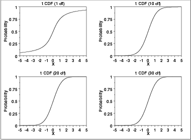
| Cumulative Distribution Function | The formula for the cumulative distribution function of the tdistribution is complicated and is not included here. It is given in theEvans, Hastings, and Peacock book.The following are the plots of the t cumulative distribution function with the same values of  as the pdf plots above. as the pdf plots above. | ||||||||||||||||
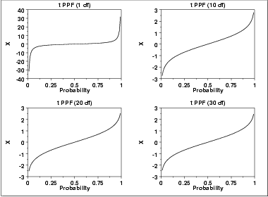
| Percent Point Function | The formula for the percent point function of the t distribution does not exist in a simple closed form. It is computed numerically.The following are the plots of the t percent point function with the same values of  as the pdf plots above. as the pdf plots above. | ||||||||||||||||
| Other Probability Functions | Since the t distribution is typically used to develop hypothesis tests and confidence intervals and rarely for modeling applications, we omit the formulas and plots for the hazard, cumulative hazard, survival, and inverse survival probability functions. | ||||||||||||||||
| Common Statistics |
| ||||||||||||||||
| Parameter Estimation | Since the t distribution is typically used to develop hypothesis tests and confidence intervals and rarely for modeling applications, we omit any discussion of parameter estimation. | ||||||||||||||||
| Comments | The t distribution is used in many cases for the critical regions for hypothesis tests and in determining confidence intervals. The most common example is testing if data are consistent with the assumed process mean. | ||||||||||||||||
| Software | Most general purpose statistical software programs support at least some of the probability functions for the t distribution. | ||||||||||||||||
Gertrude Cox : Gertrude Mary Cox (of Experimental Statistics at North Carolina State University. She was later appointed director of both the Institute of Statistics of 1900 - 1978) was an influential American statistician and founder of the department the Consolidated University of North Carolina and the Statistics Research Division of North Carolina State University. Her most important and influential research dealt with experimental design; she wrote an important book on the subject with W. G. Cochran. In 1949 Cox became the first female elected into the International Statistical Institute and in 1956 she was president of the American Statistical Association. From 1931 to 1933 Cox undertook graduate studies in statistics at the University of California at Berkeley , then returned to Iowa State College as assistant in the Statistical Laboratory. Here she worked on the design of experiments . In 1939 she was appointed assistant professor of statisti...
 It is undefined for
  It is undefined for
Comments
Post a Comment