| |||||||||||||
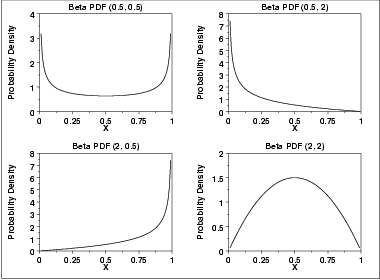
| Probability Density Function | The general formula for the probability density function of the beta distribution is where p and q are the shape parameters, a and b are the lower and upper bounds, respectively, of the distribution, and B(p,q) is the beta function. The beta function has the formula ![B(alpha,beta) = INTEGRAL[0 to 1][t^(alpha-1)*(1-t)^(beta-1)dt]](http://www.itl.nist.gov/div898/handbook/eda/section3/eqns/betafunc.gif) The case where a = 0 and b = 1 is called the standard beta distribution. The equation for the standard beta distribution is  Typically we define the general form of a distribution in terms of location and scale parameters. The beta is different in that we define the general distribution in terms of the lower and upper bounds. However, the location and scale parameters can be defined in terms of the lower and upper limits as follows:
scale = b - a  | ||||||||||||
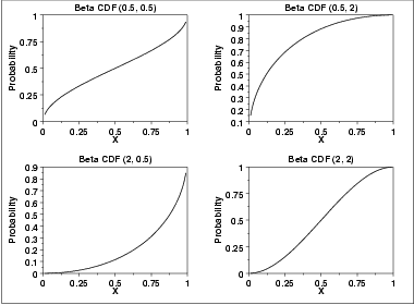
| Cumulative Distribution Function | The formula for the cumulative distribution function of the beta distribution is also called the incomplete beta function ratio (commonly denoted by Ix) and is defined as![F(x) = I(x)(p,q) =
(1/B(p,q))*INTEGRAL[0 to x][t^(p-1)*(1-t)^(q-1) dt](http://www.itl.nist.gov/div898/handbook/eda/section3/eqns/betcdf.gif)  | ||||||||||||
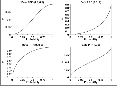
| Percent Point Function | The formula for the percent point function of the beta distribution does not exist in a simple closed form. It is computed numerically.The following is the plot of the beta percent point function with the same values of the shape parameters as the pdf plots above. | ||||||||||||
| Other Probability Functions | Since the beta distribution is not typically used for reliability applications, we omit the formulas and plots for the hazard, cumulative hazard, survival, and inverse survival probability functions. | ||||||||||||
| Common Statistics | The formulas below are for the case where the lower limit is zero and the upper limit is one.
| ||||||||||||
| Parameter Estimation | First consider the case where a and b are assumed to be known. For this case, the method of moments estimates are![p = xbar*[(xbar*(1-xbar)/s^2) - 1]](http://www.itl.nist.gov/div898/handbook/eda/section3/eqns/betamom1.gif) ![p = xbar*[(xbar*(1-xbar)/s^2) - 1]](http://www.itl.nist.gov/div898/handbook/eda/section3/eqns/betamom2.gif)  is the sample mean and s2 is the sample variance. If a and b are not 0 and 1, respectively, then replace is the sample mean and s2 is the sample variance. If a and b are not 0 and 1, respectively, then replace  with with  and s2 with and s2 with  in the above equations.For the case when a and b are known, the maximum likelihood estimates can be obtained by solving the following set of equations in the above equations.For the case when a and b are known, the maximum likelihood estimates can be obtained by solving the following set of equations![psi(phat)-psi(phat+qhat)=(1/n)*SUM[i=1 to n][LOG[(Y(i)-b)/(b-a)]]](http://www.itl.nist.gov/div898/handbook/eda/section3/eqns/betaml1.gif) ![psi(phat)-psi(phat+qhat)=(1/n)*SUM[i=1 to n][LOG[(Y(i)-b)/(b-a)]]](http://www.itl.nist.gov/div898/handbook/eda/section3/eqns/betaml2.gif) | ||||||||||||
| Software | Most general purpose statistical software programs support at least some of the probability functions for the beta distribution. | ||||||||||||
Gertrude Cox : Gertrude Mary Cox (of Experimental Statistics at North Carolina State University. She was later appointed director of both the Institute of Statistics of 1900 - 1978) was an influential American statistician and founder of the department the Consolidated University of North Carolina and the Statistics Research Division of North Carolina State University. Her most important and influential research dealt with experimental design; she wrote an important book on the subject with W. G. Cochran. In 1949 Cox became the first female elected into the International Statistical Institute and in 1956 she was president of the American Statistical Association. From 1931 to 1933 Cox undertook graduate studies in statistics at the University of California at Berkeley , then returned to Iowa State College as assistant in the Statistical Laboratory. Here she worked on the design of experiments . In 1939 she was appointed assistant professor of statisti...


![SQRT[(p*q)/((p+q)^2*(p+q+1))]](http://www.itl.nist.gov/div898/handbook/eda/section3/eqns/betasd.gif)

![SQRT[2*(q-p)*(SQRT(p+q+1)]/[(p+q+2)*SQRT(p*q)]](http://www.itl.nist.gov/div898/handbook/eda/section3/eqns/betaskew.gif)
Comments
Post a Comment