| |||||||||||||||||
| Probability Density Function | The general formula for the probability density function of the exponential distribution is where  is the location parameter and is the location parameter and  is the scale parameter(the scale parameter is often referred to as is the scale parameter(the scale parameter is often referred to as  which equals which equals  ). The case where ). The case where  = 0 and = 0 and  = 1 is called the standard exponential distribution. The equation for the standard exponential distribution is = 1 is called the standard exponential distribution. The equation for the standard exponential distribution is The general form of probability functions can be expressed in terms of the standard distribution. Subsequent formulas in this section are given for the 1-parameter (i.e., with scale parameter) form of the function. The following is the plot of the exponential probability density function. 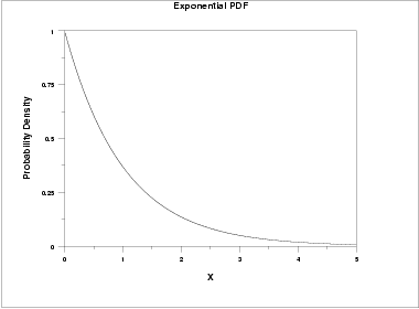 | ||||||||||||||||
| Cumulative Distribution Function | The formula for the cumulative distribution function of the exponential distribution is The following is the plot of the exponential cumulative distribution function. 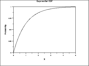 | ||||||||||||||||
| Percent Point Function | The formula for the percent point function of the exponential distribution is The following is the plot of the exponential percent point function. 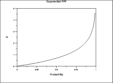 | ||||||||||||||||
| Hazard Function | The formula for the hazard function of the exponential distribution is The following is the plot of the exponential hazard function. 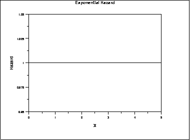 | ||||||||||||||||
| Cumulative Hazard Function | The formula for the cumulative hazard function of the exponential distribution is The following is the plot of the exponential cumulative hazard function. 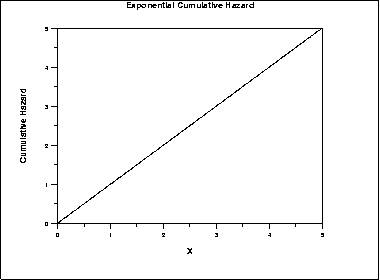 | ||||||||||||||||
| Survival Function | The formula for the survival function of the exponential distribution is The following is the plot of the exponential survival function. 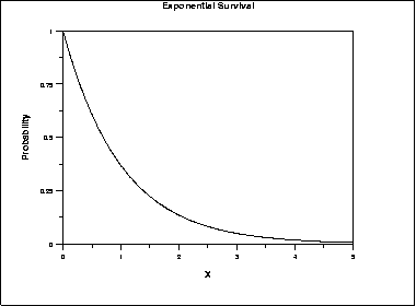 | ||||||||||||||||
| Inverse Survival Function | The formula for the inverse survival function of the exponential distribution is The following is the plot of the exponential inverse survival function. 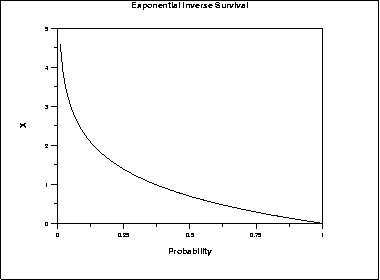 | ||||||||||||||||
| Common Statistics |
| ||||||||||||||||
| Parameter Estimation | For the full sample case, the maximum likelihood estimator of the scale parameter is the sample mean. Maximum likelihood estimation for the exponential distribution is discussed in the chapter on reliability (Chapter 8). It is also discussed in chapter 19 of Johnson, Kotz, and Balakrishnan. | ||||||||||||||||
| Comments | The exponential distribution is primarily used in reliabilityapplications. The exponential distribution is used to model data with a constant failure rate (indicated by the hazard plot which is simply equal to a constant). | ||||||||||||||||
| Software | Most general purpose statistical software programs support at least some of the probability functions for the exponential distribution | ||||||||||||||||
Gertrude Cox : Gertrude Mary Cox (of Experimental Statistics at North Carolina State University. She was later appointed director of both the Institute of Statistics of 1900 - 1978) was an influential American statistician and founder of the department the Consolidated University of North Carolina and the Statistics Research Division of North Carolina State University. Her most important and influential research dealt with experimental design; she wrote an important book on the subject with W. G. Cochran. In 1949 Cox became the first female elected into the International Statistical Institute and in 1956 she was president of the American Statistical Association. From 1931 to 1933 Cox undertook graduate studies in statistics at the University of California at Berkeley , then returned to Iowa State College as assistant in the Statistical Laboratory. Here she worked on the design of experiments . In 1939 she was appointed assistant professor of statisti...

Comments
Post a Comment