| |||||||||||||
| Probability Density Function | The F distribution is the ratio of two chi-square distributions with degrees of freedom  and and  , respectively, where each chi-square has first been divided by its degrees of freedom. The formula for the probability density function of the F distribution is , respectively, where each chi-square has first been divided by its degrees of freedom. The formula for the probability density function of the F distribution is![[GAMMA((nu1+nu2)/2)*(nu1/nu2)**(nu1/2)*x**((nu2/2)-1)]/
GAMMA(nu1/2)*GAMMA(nu2/2)*(1 + Nu1*x/Nu2)**((nu1+nu2)/2)]](http://www.itl.nist.gov/div898/handbook/eda/section3/eqns/fpdf.gif)  and and  are the shape parameters and are the shape parameters and  is the gamma function. The formula for the gamma function is is the gamma function. The formula for the gamma function is![GAMMA(a) = INTEGRAL[t**(a-1)*EXP(-t)dt] where the
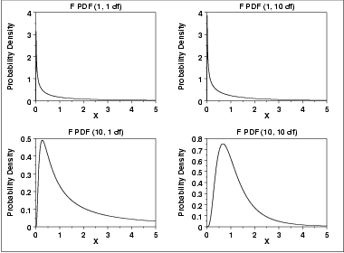
integration is from 0 to infinity](http://www.itl.nist.gov/div898/handbook/eda/section3/eqns/gammfunc.gif)  , and a scale parameter, , and a scale parameter,  .The following is the plot of the F probability density function for 4 different values of the shape parameters. .The following is the plot of the F probability density function for 4 different values of the shape parameters. | ||||||||||||
| Cumulative Distribution Function | The formula for the Cumulative distribution function of the F distribution is  / ( / ( + +  *x) and Ik is the incomplete beta function. The formula for the incomplete beta function is *x) and Ik is the incomplete beta function. The formula for the incomplete beta function is![I(k)(x,alpha,beta) = INTEGRAL[t**(alpha-1)*(1-t)**(beta-1)dt]/
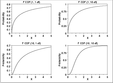
B(alpha,beta) where the integration is from 0 to x](http://www.itl.nist.gov/div898/handbook/eda/section3/eqns/ibetfunc.gif)   and and  as the pdf plots above. as the pdf plots above. | ||||||||||||
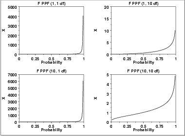
| Percent Point Function | The formula for the percent point function of the F distribution does not exist in a simple closed form. It is computed numerically.The following is the plot of the F percent point function with the same values of  and and  as the pdf plots above. as the pdf plots above. | ||||||||||||
| Other Probability Functions | Since the F distribution is typically used to develop hypothesis tests and confidence intervals and rarely for modeling applications, we omit the formulas and plots for the hazard, cumulative hazard, survival, and inverse survival probability functions. | ||||||||||||
| Common Statistics | The formulas below are for the case where the location parameter is zero and the scale parameter is one.
| ||||||||||||
| Parameter Estimation | Since the F distribution is typically used to develop hypothesis tests and confidence intervals and rarely for modeling applications, we omit any discussion of parameter estimation. | ||||||||||||
| Comments | The F distribution is used in many cases for the critical regions for hypothesis tests and in determining confidence intervals. Two common examples are the analysis of variance and the F test to determine if the variances of two populations are equal. | ||||||||||||
| Software | Most general purpose statistical software programs support at least some of the probability functions for the F distribution | ||||||||||||
Gertrude Cox : Gertrude Mary Cox (of Experimental Statistics at North Carolina State University. She was later appointed director of both the Institute of Statistics of 1900 - 1978) was an influential American statistician and founder of the department the Consolidated University of North Carolina and the Statistics Research Division of North Carolina State University. Her most important and influential research dealt with experimental design; she wrote an important book on the subject with W. G. Cochran. In 1949 Cox became the first female elected into the International Statistical Institute and in 1956 she was president of the American Statistical Association. From 1931 to 1933 Cox undertook graduate studies in statistics at the University of California at Berkeley , then returned to Iowa State College as assistant in the Statistical Laboratory. Here she worked on the design of experiments . In 1939 she was appointed assistant professor of statisti...


Comments
Post a Comment