| |||||||||||||||||
| Probability Density Function | The general formula for the probability density function of the normal distribution is![f(x) = EXP[-(x-mu)**2/(2*sigma**2)]/(sigma*SQRT(2*PI))](http://www.itl.nist.gov/div898/handbook/eda/section3/eqns/norpdfg.gif) where  is the location parameter and is the location parameter and  is the scale parameter. The case where is the scale parameter. The case where  = 0 and = 0 and  = 1 is called the standard normal distribution. The equation for the standard normal distribution is = 1 is called the standard normal distribution. The equation for the standard normal distribution is![f(x) = EXP[-x**2/2]/SQRT(2*PI)](http://www.itl.nist.gov/div898/handbook/eda/section3/eqns/norpdf.gif) Since the general form of probability functions can be expressed in terms of the standard distribution, all subsequent formulas in this section are given for the standard form of the function. The following is the plot of the standard normal probability density function. 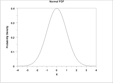 | ||||||||||||||||
| Cumulative Distribution Function | The formula for the cumulative distribution function of the normal distribution does not exist in a simple closed formula. It is computed numerically.The following is the plot of the normal cumulative distribution function.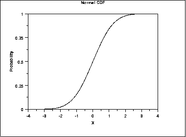 | ||||||||||||||||
| Percent Point Function | The formula for the percent point function of the normal distribution does not exist in a simple closed formula. It is computed numerically.The following is the plot of the normal percent point function.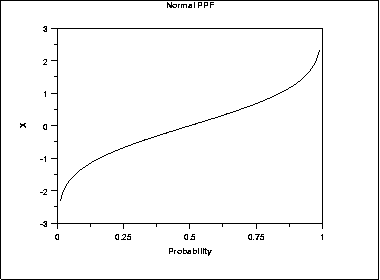 | ||||||||||||||||
| Hazard Function | The formula for the hazard function of the normal distribution is where  is the cumulative distribution function of the standardnormal distribution and is the cumulative distribution function of the standardnormal distribution and  is the probability density function of the standard normal distribution. is the probability density function of the standard normal distribution.The following is the plot of the normal hazard function. 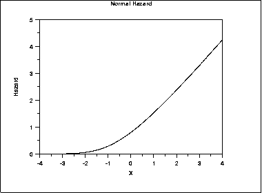 | ||||||||||||||||
| Cumulative Hazard Function | The normal cumulative hazard function can be computed from the normal cumulative distribution function.The following is the plot of the normal cumulative hazard function.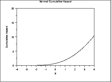 | ||||||||||||||||
| Survival Function | The normal survival function can be computed from the normal cumulative distribution function.The following is the plot of the normal survival function.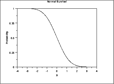 | ||||||||||||||||
| Inverse Survival Function | The normal inverse survival function can be computed from the normal percent point function.The following is the plot of the normal inverse survival function.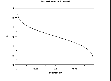 | ||||||||||||||||
| Common Statistics |
| ||||||||||||||||
| Parameter Estimation | The location and scale parameters of the normal distribution can be estimated with the sample mean and sample standard deviation, respectively. | ||||||||||||||||
| Comments | For both theoretical and practical reasons, the normal distribution is probably the most important distribution in statistics. For example,
| ||||||||||||||||
| Theroretical Justification - Central Limit Theorem | The normal distribution is widely used. Part of the appeal is that it is well behaved and mathematically tractable. However, the central limit theorem provides a theoretical basis for why it has wide applicability.The central limit theorem basically states that as the sample size (N) becomes large, the following occur:
| ||||||||||||||||
| Software | Most general purpose statistical software programs support at least some of the probability functions for the normal distribution. | ||||||||||||||||
Gertrude Cox : Gertrude Mary Cox (of Experimental Statistics at North Carolina State University. She was later appointed director of both the Institute of Statistics of 1900 - 1978) was an influential American statistician and founder of the department the Consolidated University of North Carolina and the Statistics Research Division of North Carolina State University. Her most important and influential research dealt with experimental design; she wrote an important book on the subject with W. G. Cochran. In 1949 Cox became the first female elected into the International Statistical Institute and in 1956 she was president of the American Statistical Association. From 1931 to 1933 Cox undertook graduate studies in statistics at the University of California at Berkeley , then returned to Iowa State College as assistant in the Statistical Laboratory. Here she worked on the design of experiments . In 1939 she was appointed assistant professor of statisti...

 .
.
Comments
Post a Comment