Lognormal Distribution | |||||||||||||||||
| Probability Density Function | A variable X is lognormally distributed if Y = LN(X) is normally distributed with "LN" denoting the natural logarithm. The general formula for the probability density function of the lognormal distribution is where  is the shape parameter, is the shape parameter,  is the location parameter and mis the scale parameter. The case where is the location parameter and mis the scale parameter. The case where  = 0 and m = 1 is called the standard lognormal distribution. The case where = 0 and m = 1 is called the standard lognormal distribution. The case where  equals zero is called the 2-parameter lognormal distribution. equals zero is called the 2-parameter lognormal distribution.The equation for the standard lognormal distribution is  Since the general form of probability functions can be expressed in terms of the standard distribution, all subsequent formulas in this section are given for the standard form of the function. The following is the plot of the lognormal probability density function for four values of  . .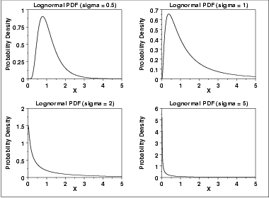 There are several common parameterizations of the lognormal distribution. The form given here is from Evans, Hastings, and Peacock. | ||||||||||||||||
| Cumulative Distribution Function | The formula for the cumulative distribution function of the lognormal distribution is where  is the cumulative distribution function of the normal distribution. is the cumulative distribution function of the normal distribution.The following is the plot of the lognormal cumulative distribution function with the same values of  as the pdf plots above. as the pdf plots above.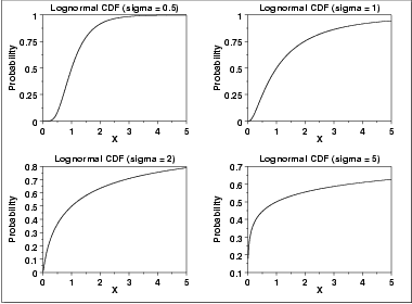 | ||||||||||||||||
| Percent Point Function | The formula for the percent point function of the lognormal distribution is where  is the percent point function of the normal distribution. is the percent point function of the normal distribution.The following is the plot of the lognormal percent point function with the same values of  as the pdf plots above. as the pdf plots above.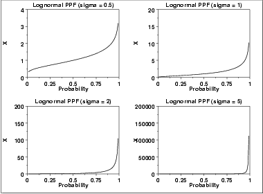 | ||||||||||||||||
| Hazard Function | The formula for the hazard function of the lognormal distribution is where  is the probability density function of the normal distributionand is the probability density function of the normal distributionand  is the cumulative distribution function of the normal distribution. is the cumulative distribution function of the normal distribution.The following is the plot of the lognormal hazard function with the same values of  as the pdf plots above. as the pdf plots above.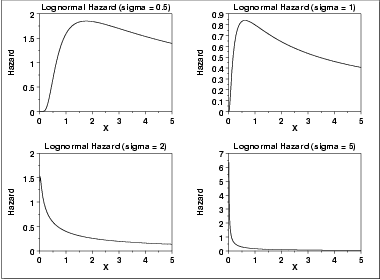 | ||||||||||||||||
| Cumulative Hazard Function | The formula for the cumulative hazard function of the lognormal distribution is where  is the cumulative distribution function of the normal distribution. is the cumulative distribution function of the normal distribution.The following is the plot of the lognormal cumulative hazard function with the same values of  as the pdf plots above. as the pdf plots above.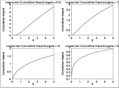 | ||||||||||||||||
| Survival Function | The formula for the survival function of the lognormal distribution is where  is the cumulative distribution function of the normal distribution. is the cumulative distribution function of the normal distribution.The following is the plot of the lognormal survival function with the same values of  as the pdf plots above. as the pdf plots above.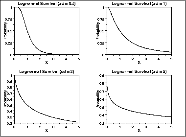 | ||||||||||||||||
| Inverse Survival Function | The formula for the inverse survival function of the lognormal distribution is where  is the percent point function of the normal distribution. is the percent point function of the normal distribution.The following is the plot of the lognormal inverse survival function with the same values of  as the pdf plots above. as the pdf plots above.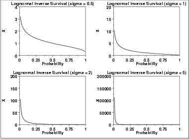 | ||||||||||||||||
| Common Statistics | The formulas below are with the location parameter equal to zero and the scale parameter equal to one.
| ||||||||||||||||
| Parameter Estimation | The maximum likelihood estimates for the scale parameter, m, and the shape parameter,  , are , are ![sigmahat = SQRT{SUM[i=1 to N][(LOG(X(i))-mu)**2]/N}](http://www.itl.nist.gov/div898/handbook/eda/section3/eqns/sigmahat.gif) ![Uhat = SUM[i=1 to N][LOG(X(i))]/N](http://www.itl.nist.gov/div898/handbook/eda/section3/eqns/uhat.gif) | ||||||||||||||||
| Comments | The lognormal distribution is used extensively in reliabilityapplications to model failure times. The lognormal and Weibulldistributions are probably the most commonly used distributions in reliability applications. | ||||||||||||||||
| Software | Most general purpose statistical software programs support at least some of the probability functions for the lognormal distribution. | ||||||||||||||||
Gertrude Cox : Gertrude Mary Cox (of Experimental Statistics at North Carolina State University. She was later appointed director of both the Institute of Statistics of 1900 - 1978) was an influential American statistician and founder of the department the Consolidated University of North Carolina and the Statistics Research Division of North Carolina State University. Her most important and influential research dealt with experimental design; she wrote an important book on the subject with W. G. Cochran. In 1949 Cox became the first female elected into the International Statistical Institute and in 1956 she was president of the American Statistical Association. From 1931 to 1933 Cox undertook graduate studies in statistics at the University of California at Berkeley , then returned to Iowa State College as assistant in the Statistical Laboratory. Here she worked on the design of experiments . In 1939 she was appointed assistant professor of statisti...


Comments
Post a Comment