Methods of correlation

Correlation Methods 

Correlation and Covariance Matrices
Fisher's z Transformation (z_r)
Pearson Product-Moment Correlation Coefficient (Pearson's r)
Spearman's Rank-Order Correlation Coefficient (Spearman's ρ)
Kendall's Rank Correlation Coefficient (Kendall's τ)



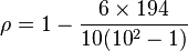
Correlation and Covariance Matrices




You can generate a correlation or covariance matrix from numeric data columns, and have the choice of storing the computation results in an-autogenerated worksheet, or display the results in a table format whose values can be color coded.

• This method requires multiple numeric data columns whose values should be stored in a single worksheet.
An example of a correlation matrix displayed as a color-coded table is shown below.





Using Fisher's z Transformation (z_r)




This option is provided to allow transforming a skewed sampling distribution into a normalized format. The theoretical sampling distribution of the correlation coefficient can be approximated by the normal distribution when the value of a population correlation ρ = 0, but as the value of r deviates from zero, the sampling distribution becomes increasingly skewed. Fisher's ztransformation transforms a skewed sampling distribution into a normalized format. The relationship between Pearson's product-moment correlation coefficient and the Fisher-Transformed values are shown in the right-hand side image. The image below shows the Fisher-transformed values of the correlation matrix displayed above.




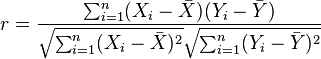
Pearson Product-Moment Correlation Coefficient (Pearson's r)







Pearson's correlation coefficient when applied to a population is commonly represented by the Greek letter ρ (rho) and may be referred to as the population correlation coefficient or thepopulation Pearson correlation coefficient. The formula for ρ is:






For a sample[edit]

Pearson's correlation coefficient when applied to a sample is commonly represented by the letter r and may be referred to as the sample correlation coefficient or the sample Pearson correlation coefficient. We can obtain a formula for r by substituting estimates of the covariances and variances based on a sample into the formula above. That formula for r is:



An equivalent expression gives the correlation coefficient as the mean of the products of the standard scores. Based on a sample of paired data (X_i, Y_i), the sample Pearson correlation coefficient is



where



are the standard score, sample mean, and sample standard deviation, respectively.

Mathematical properties[edit]

The absolute value of both the sample and population Pearson correlation coefficients are less than or equal to 1. Correlations equal to 1 or -1 correspond to data points lying exactly on a line (in the case of the sample correlation), or to a bivariate distribution entirely supported on a line (in the case of the population correlation). The Pearson correlation coefficient is symmetric: corr(X,Y) = corr(Y,X).

A key mathematical property of the Pearson correlation coefficient is that it is invariant (up to a sign) to separate changes in location and scale in the two variables. That is, we may transform X to a + bX and transform Y to c + dY, where a, b, c, and d are constants, without changing the correlation coefficient (this fact holds for both the population and sample Pearson correlation coefficients). Note that more general linear transformations do change the correlation: see a later section for an application of this.

The Pearson correlation can be expressed in terms of uncentered moments. Since μ_X = E(X), σ_X² = E[(X − E(X))²] = E(X²) − E²(X) and likewise for Y, and since



the correlation can also be written as



Spearman's rank correlation coefficient




In applications where duplicate values (ties) are known to be absent, a simpler procedure can be used to calculate ρ.^[3][4]Differences  between the ranks of each observation on the two variables are calculated, and ρ is given by:



Note that this latter method should not be used in cases where the data set is truncated; that is, when the Spearman correlation coefficient is desired for the top X records (whether by pre-change rank or post-change rank, or both), the user should use the Pearson correlation coefficient formula given above.

Example [edit]

In this example, we will use the raw data in the table below to calculate the correlation between the IQ of a person with the number of hours spent in front of TV per week.

IQ,	Hours of TV per week,
106	7
86	0
100	27
101	50
99	28
103	29
97	20
113	12
112	6
110	17

First, we must find the value of the term . To do so we use the following steps, reflected in the table below.

1. Sort the data by the first column (). Create a new column  and assign it the ranked values 1,2,3,...n.
2. Next, sort the data by the second column (). Create a fourth column  and similarly assign it the ranked values 1,2,3,...n.
3. Create a fifth column  to hold the differences between the two rank columns ( and ).
4. Create one final column  to hold the value of column  squared.

IQ,	Hours of TV per week,	rank	rank
86	0	1	1	0	0
97	20	2	6	−4	16
99	28	3	8	−5	25
100	27	4	7	−3	9
101	50	5	10	−5	25
103	29	6	9	−3	9
106	7	7	3	4	16
110	17	8	5	3	9
112	6	9	2	7	49
113	12	10	4	6	36

With  found, we can add them to find . The value of n is 10. So these values can now be substituted back into the equation,



which evaluates to ρ = -29/165 = −0.175757575... with a P-value = 0.6864058 (using the t distribution)

This low value shows that the correlation between IQ and hours spent watching TV is very low.